Multirate filters are digital filters that change the sample rate of an sampled input signal. The process of rate conversion involves an upsampler, a downsampler, and a lowpass filter to process the signal.
The most basic multirate filters are interpolators, decimators, and noninteger sample rate converters. These filters are building components of more advanced filter technologies such as channelizers, channel synthesizers, two-channel filter banks, and Quadrature Mirror Filter (QMF). You can design these filters in MATLAB® and Simulink® using the designMultirateFIR function.
The designMultirateFIR function automatically designs an anti-aliasing FIR filter based on the rate conversion factor that you specify. The inputs to the designMultirateFIR function are the interpolation factor and the decimation factor. Optionally, you can provide the half-polyphase length or transition width and stopband attenuation. To design a decimator, set the interpolation factor to 1. Similarly, to design an interpolator, set the decimation factor to 1.
To implement the multirate filters in MATLAB, use the coefficients returned by the designMultirateFIR function as inputs to the dsp.FIRDecimator, dsp.FIRInterpolator, and dsp.FIRRateConverter System objects.
b = designMultirateFIR(1,4);
firDecim = dsp.FIRDecimator(4,b)
firDecim =

  dsp.FIRDecimator with properties:

    DecimationFactor: 4
     NumeratorSource: 'Property'
           Numerator: [0 -2.2355e-05 -5.0269e-05 -5.2794e-05 0 1.0256e-04 1.9352e-04 … ]
           Structure: 'Direct form'
Alternatively, you can set the SystemObject flag of the designMultirateFIR function to true. The function designs and automatically creates the appropriate rate conversion object.
firDecim = designMultirateFIR(1,4,'SystemObject',true)
firDecim =

  dsp.FIRDecimator with properties:

    DecimationFactor: 4
     NumeratorSource: 'Property'
           Numerator: [0 -2.2355e-05 -5.0269e-05 -5.2794e-05 0 1.0256e-04 1.9352e-04 … ]
           Structure: 'Direct form'
In Simulink, compute these coefficients using the designMultirateFIR function in the default Auto mode of the FIR Decimation, FIR Interpolation, and FIR Rate Conversion blocks. You can also specify these coefficients as parameters or pass them through an input port.
These examples show how to implement an FIR decimator in MATLAB and Simulink. You can apply this workflow to an FIR interpolator and FIR rate converter as well.
Implement an FIR Decimator in MATLAB
To implement an FIR Decimator, you must first design it by using the designMultirateFIR function. Specify the decimation factor of interest (usually greater than 1) and an interpolation factor equal to 1. You can use the default half-polyphase length of 12 and the default stopband attenuation of 80 dB. Alternatively, you can also specify the half-polyphase length, transition width, and stopband attenuation values.
Design an FIR decimator with the decimation factor set to 3 and the half-polyphase length set to 14. Use the default stopband attenuation of 80 dB.
b = designMultirateFIR(1,3,14);
Provide the coefficients vector b as an input to the dsp.FIRDecimator System object™.
firDecim = dsp.FIRDecimator(3,b);
fvtool(firDecim)
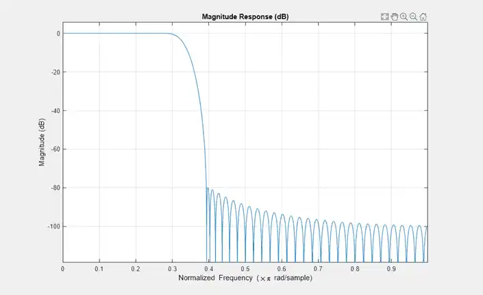
By default, the fvtool function shows the magnitude response. Navigate through the Filter Visualization Tool toolbar to see the phase response, impulse response, group delay, and other filter analysis information.
Filter a noisy sine wave input using the firDecim object. The sine wave has frequencies at 1000 Hz and 3000 Hz. The noise is a white Gaussian noise with zero mean and a standard deviation of 1e-5. The decimated output will have one-third the sample rate as the input. Initialize two spectrumAnalyzer objects, one for the input and the other for the output.
f1 = 1000;
f2 = 3000;
Fs = 8000;
source = dsp.SineWave('Frequency',[f1,f2],'SampleRate',Fs,...
    'SamplesPerFrame',1026);

specanainput = spectrumAnalyzer('SampleRate',Fs,...
    'PlotAsTwoSidedSpectrum',false,...
    'Method','welch',...
    'ShowLegend',true,'YLimits',[-120 40],...
    'Title','Noisy Input signal',...
    'ChannelNames', {'Noisy Input'});
specanaoutput = spectrumAnalyzer('SampleRate',Fs/3,...
    'PlotAsTwoSidedSpectrum',false,...
    'Method','welch',...
    'ShowLegend',true,'YLimits',[-120 40],...
    'Title','Filtered output',...
    'ChannelNames', {'Filtered output'});
Stream the input and filter it in a processing loop.
Note: If you are using R2016a or an earlier release, replace each call to the object with the equivalent step syntax. For example, obj(x) becomes step(obj,x).
for Iter = 1:1000
    input = sum(source(),2);
    noisyInput = input + (10^-5)*randn(1026,1);
    output = firDecim(noisyInput);
    specanainput(noisyInput)
    specanaoutput(output)
end
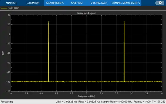
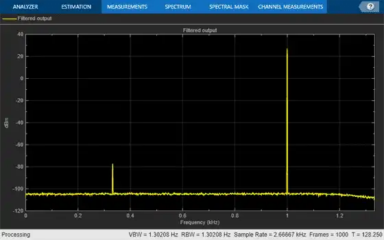
The input has two peaks: one at 1000 Hz and the other at 3000 Hz. The filter has a lowpass response with a passband frequency of 0.3π rad/sample. With a sample rate of 8000 Hz, that value is a passband frequency of 1200 Hz. The tone at 1000 Hz is unattenuated because it falls in the passband of the filter. The tone at 3000 Hz is filtered out.
Similarly, you can design an FIR interpolator and an FIR rate Converter by providing appropriate inputs to the designMultirateFIR function. To implement the filters, pass the designed coefficients to the dsp.FIRInterpolator and dsp.FIRRateConverter objects.
Implement an FIR Decimator in Simulink
You can design and implement the FIR multirate filters in Simulink™ using the FIR Decimation, FIR Interpolation, and FIR Rate Conversion blocks.
Open the model 'multiratefiltering.slx'.
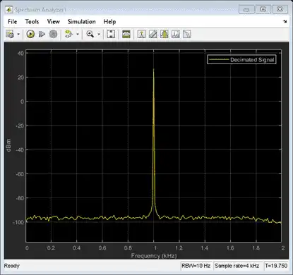
The input signal is a noisy sinusoidal signal with two frequencies: one at 1000 Hz and the other at 3000 Hz. The sample rate of the signal is 8000 Hz and the Samples per frame parameter of the Sine Wave blocks is set to 1026. The noise added to the signal is a white Gaussian noise with zero mean and a variance of 1e-10.
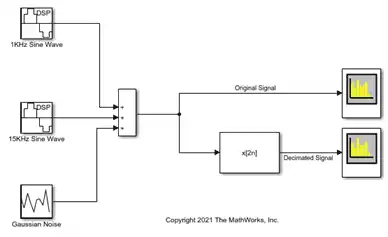
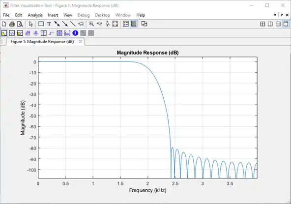
The Coefficient source parameter of the FIR Decimation block is set to Dialog parameters, and the FIR filter coefficients parameter is set to designMultirateFIR(1,2). The function uses the default half-polyphase length of 12 and the default stopband attenuation of 80 dB. The magnitude response of the designed filter looks like as follows:
Run the model.
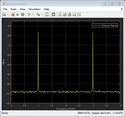
The first spectrum analyzer shows the spectrum of the original signal, while the second spectrum analyzer shows the spectrum of the decimated signal. Because the Rate options parameter in the FIR Decimation block is set to Allow multirate processing, the frame size of the signal is the same at the input and output of the FIR Decimation block, while the sample rate changes. For more details on this mode, see Rate Conversion by Frame-Rate Adjustment.
Sample Rate Conversion
Sample rate conversion is a process of converting the sample rate of a signal from one sampling rate to another sampling rate. Multistage filters minimize the amount of computation involved in sample rate conversion. To perform an efficient multistage rate conversion, use the dsp.SampleRateConverter object that:
-
Accepts input sample rate and output sample rate as inputs.
-
Partitions the design problem into optimal stages.
-
Designs all the filters required by the various stages.
-
Implements the design.
The design makes sure that aliasing does not occur in the intermediate steps.
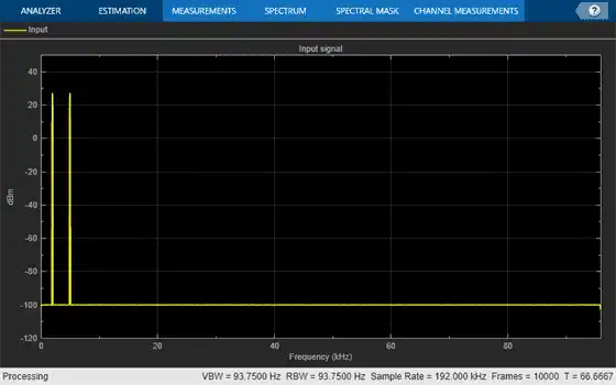
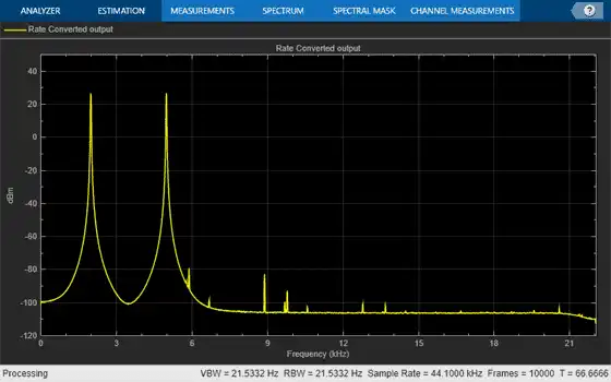
In this example, change the sample rate of a noisy sine wave signal from an input rate of 192 kHz to an output rate of 44.1 kHz.
Initialize a sample rate converter object.
SRC = dsp.SampleRateConverter;
Display the filter information.
info(SRC)
ans =
    'Overall Interpolation Factor    : 147
     Overall Decimation Factor       : 640
     Number of Filters               : 3
     Multiplications per Input Sample: 27.667188
     Number of Coefficients          : 8631
     Filters:
        Filter 1:
        dsp.FIRDecimator     - Decimation Factor   : 2
        Filter 2:
        dsp.FIRDecimator     - Decimation Factor   : 2
        Filter 3:
        dsp.FIRRateConverter - Interpolation Factor: 147
                             - Decimation Factor   : 160
     '
SRC is a three-stage filter: two FIR decimators followed by an FIR rate converter.
Initialize the sine wave source. The sine wave has two tones: one at 2000 Hz and the other at 5000 Hz.
source = dsp.SineWave ('Frequency',[2000 5000],'SampleRate',192000,...
    'SamplesPerFrame',1280);
Initialize two spectrum analyzers, one to see the spectrum of the input signal and the other to see the spectrum of the rate converted output signal. The 'PlotAsTwoSidedSpectrum' property of the spectrumAnalyzer objects is set to 'false', indicating that the spectrum shown is one-sided in the range [0 Fs/2], where Fs is the sample rate of the signal.
Fsin = SRC.InputSampleRate;
Fsout = SRC.OutputSampleRate;
specanainput = spectrumAnalyzer('SampleRate',Fsin,...
    'PlotAsTwoSidedSpectrum',false,...
    'Method','welch',...
    'ShowLegend',true,'YLimits',[-120 50],...
    'Title','Input signal',...
    'ChannelNames', {'Input'});
specanaoutput = spectrumAnalyzer('SampleRate',Fsout,...
    'PlotAsTwoSidedSpectrum',false,...
    'Method','welch',...
    'ShowLegend',true,'YLimits',[-120 50],...
    'Title','Rate Converted output',...
    'ChannelNames', {'Rate Converted output'});
Stream the input signal and convert the sample rate of the signal using the sample rate converter. View the spectra of both the input and output signals in the two spectrum analyzers.
The spectrum analyzers show the spectrum in the range [0 Fs/2]. For the spectrum analyzer showing the input, Fs/2 is 192000/2. For the spectrum analyzer showing the output, Fs/2 is 44100/2. Hence, the sample rate of the signal changes from 192 kHz to 44.1 kHz.
for Iter = 1:10000
    input = sum(source(),2);
    noisyinput = input + (10^-5)*randn(1280,1);
    output = SRC(noisyinput);
    specanainput(noisyinput);
    specanaoutput(output);
end
