Thermal Analysis sample
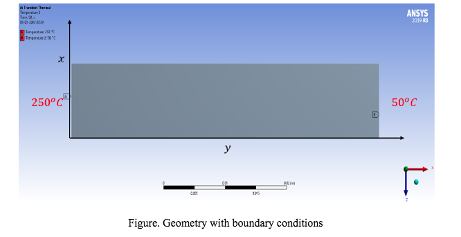
Investigate a one dimensional transient heat conduction along a 5 cm long steel bar. The initial temperature of the bar is 50 deg C and one end of the bar is held at this temperature. The other side of the bar is suddenly brought into contact with a surface at 250 deg C. Develop a finite difference model of transient one dimensional heat transfer and use this model to show how the temperature along the bar changes with time. The model can be developed using a spreadsheet or coded in python or MATLAB. Compare these results with a simple model produced in ANSYS Transient Thermal.
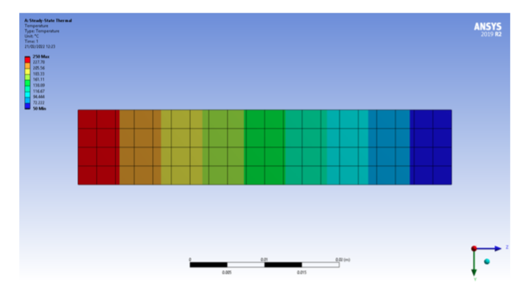
Table 1: Data for heat transfer investigation.
| Hot Side T [0C] | Cold Side T [0C] | Thermal Conductivity [W/m.K] | Thermal Capacity [kJ/kg.K] | Material Density [kg/m3] | Time step [s] |
| 250 | 50 | 54 | 0.465 | 7750 | 0.5 |
Answer
Introduction
In this task we are going to investigate a one-dimensional transient heat conduction along a 5cm long steel bar with the initial temperature of bar is 50 degrees Celsius and end of the bar is held on the same temperature, the other side of the end is contact with the surface whose temperature is 250 degrees Celsius. Finite-difference methods are a group of numerical approaches for solving differential equations using finite differences to approximate derivatives. The value of the solution at these discrete places is approximated by solving algebraic equations including finite differences and values from neighbouring points, and the geographic domain and time interval are both discretized, or broken into a finite number of steps. We derive the finite difference model for transient one-dimensional heat transfer equation and solve the partial derivate heat equation using the FDM approach, we also do the same transient analysis on the ANSYS to verify the output result of the implemented FD Model, the formulation one dimensional transient heat equation is given below
Tt=2Tx2
Whereas
α=kcp
k is the thermal conductivity
is the density of material
cp is Heat capacity
Solving the above expression using the finite difference method to compute the temperature distribution across the length for time step of 0.5 seconds, the geometry of the bar with the two-boundary conditions is shown below,
Finite Difference Model
We develop the model of the one-dimension transient heat equation using the finite difference method with the help of Partial derivative heat equation for steel bar. First step in the FDM is to discretise the model into equal step size data in spatial and time domain, for the computation we have taken time step of 0.5 seconds and step length of 0.005m, the PED heat equation is given as

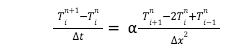
Now in finite difference method the continuous derivative equation is converted into the finite difference approximation. The derivative of temperature with respect to time can be approximated with a forward finite difference approximation as

The spatial derivative i.e., the derivative of temperature with respect to length of bar is replaced by the central finite difference approximation as

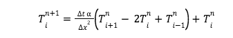
Now substituting the above finite difference approximation into the PDE equation to get the Finite Difference analogue, we get
The temperature for the next time step Tin+1 is
Boundary condition are

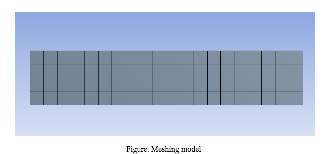
Whereas for the above BC’s i is the last node of the discretise model. To verify the model, we also model the bar in ANSYS and run the simulation for the Transient Heat Transfer analysis for the initial and boundary condition. First, we model the geometry of the model using the space claim tool in ANSYS with the length of bar as 5cm long. After that we mesh the model with the square grids here if we used the finer mesh grid then the solution of the model will give us the accurate result, assignment of the material for the given heat transfer properties that described in the problem statement. the meshing result of the ANSYS based model is shown below
We apply the transient thermal boundary condition to the model and compute the solution for 50 seconds. Now we solve the above expression for the one-dimensional transient heat equation using the finite difference approach in MATLAB and plot the temperature distribution across the length of the bar for final time of 50 seconds with the time step of 0.5 seconds. The data required for the heat transfer investigation is given below