How do I get smooth edges for a contourf plot on a log-log scale scatterplot?

Hello, I am having some trouble with using the contourf function on a log-log scale plot. I have 9 datapoints in a 2D scatterplot that are colored for a third variable. The code I use to plot the data as well as the plot are included below. a = reshape(mtot_1,1,[]); % convert matrix to row vector b = reshape(MFR_1,1,[]); % convert matrix to row vector c = reshape(SN_maxes_1,1,[]); % convert matrix to row vector figure(4) clf hold on scatter(b, a, [], c, 'filled') set(gca,'xscale','log') set(gca,'yscale','log') colorbar xlabel('MFR') ylabel('total mass flow') As you can see, on a log-log scale, the datapoits form a sort of "skewed quadrilateral" shape with edges that look "straight" when plotted on log-log. I want to create a contour map from these 9 points, but when I do, it looks like the plot below because the contour is generated with a linear interpolation method that creates straight lines between the points on a normal linear axis scale, which then look distorted or curved when plotted on the log-log scale. I have also included the code I use. figure(5) clf hold on contourf(MFR_1, mtot_1, SN_maxes_1, 100, 'LineStyle', 'none') scatter(b, a, [], c, 'filled') set(gca,'xscale','log') set(gca,'yscale','log') d = colorbar; d.Label.String = "Swirl No."; xlabel('MFR') ylabel('total mass flow') I would like to make it so that the contour plot has "straight" edges between the outer datapoints when plotted on the log-log scale, so that the contour map essentially appears as a quadrilateral with straight sides on the log-log plot instead of the odd curvy shape in the contour plot above. Can someone please offer me some advice as to how to achieve this? Thanks in advance!
 John Michell answered .
2025-11-20
John Michell answered .
2025-11-20
MFR_1 = [0.93016, 0.13933, 0.04154; 4.75072, 0.96454, 0.27638; 16.1767, 3.35929, 1.03684];
%Then the y-axis data (also a matrix):
mtot_1 = [0.00087393, 0.001293, 0.00161739; 0.00146412, 0.00182395, 0.00211802; 0.00195069, 0.00228598, 0.002528465];
%Then the "z" data (if you would call it that). This is what determines the color of the dots. It is also a matrix:
SN_maxes_1 = [1.678801, 1.627564, 1.521288; 1.535838, 1.848008, 1.7666569; 1.419559, 1.818278, 1.963394];
a = reshape(mtot_1,1,[]); % convert matrix to row vector
b = reshape(MFR_1,1,[]); % convert matrix to row vector
c = reshape(SN_maxes_1,1,[]); % convert matrix to row vector
figure(4)
clf
hold on
scatter(b, a, [], c, 'filled')
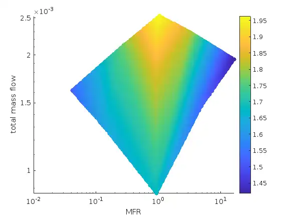
% create a mesh with constant log spacing , and find points that are inside
% a polygon (convex hull)
bl = log10(b');
al = log10(a');
cl = log10(c');
k = boundary(bl,al,1); % define outer hull
xv = bl(k);
yv = al(k);
% plot(10.^xv, 10.^yv, '-r')
x = linspace(min(xv),max(xv),200);
y = linspace(min(yv),max(yv),200);
[X,Y] = meshgrid(x,y);
x = X(:);
y = Y(:);
in = inpolygon(x,y,xv,yv);
xin = 10.^(X(in));
yin = 10.^(Y(in));
vq = griddata(bl,al,c,log10(xin),log10(yin));
scatter(xin, yin, [], vq, 'filled')
% plot(xin,yin,'.r')
set(gca,'xscale','log')
set(gca,'yscale','log')
colorbar
xlabel('MFR')
ylabel('total mass flow')
hold off