In practice, “applying machine learning” means that you apply an algorithm to data, and that algorithm creates a model that captures the trends in the data. There are many different types of machine learning models to choose from, and each has its own characteristics that may make it more or less appropriate for a given dataset.
This page gives an overview of different types of machine learning models available for supervised learning; that is, for problems where we build a model to predict a response. Within supervised learning there are two categories of models: regression (when the response is continuous) and classification (when the response belongs to a set of classes).
Popular Machine Learning Models for Regression
| Model | Image | How It Works | MATLAB Function | Further Reading |
|---|---|---|---|---|
| Linear Regression | 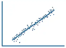 |
Linear regression is a statistical modeling technique used to describe a continuous response variable as a linear function of one or more predictor variables. Because linear regression models are simple to interpret and easy to train, they are often the first models to be fitted to a new dataset. | fitlm |
What Is a Linear Regression Model? (Documentation) Fitting a Linear Regression Machine Learning Model (Code Example) |
| Nonlinear Regression | 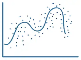 |
Nonlinear regression is a statistical modeling technique that helps describe nonlinear relationships in experimental data. Nonlinear regression models are generally assumed to be parametric, where the model is described as a nonlinear equation. “Nonlinear” refers to a fit function that is a nonlinear function of the parameters. For example, if the fitting parameters are b0, b1, and b2: the equation y = b0+b1x+b2x2 is a linear function of the fitting parameters, whereas y = (b0xb1)/(x+b2) is a nonlinear function of the fitting parameters. |
fitnlm |
Nonlinear Regression (Documentation) Fitting a Nonlinear Regression Machine Learning Model (Code Example) |
| Gaussian Process Regression (GPR) | 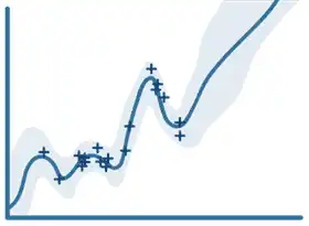 |
GPR models are nonparametric machine learning models that are used for predicting the value of a continuous response variable. The response variable is modeled as a Gaussian process, using covariances with the input variables. These models are widely used in the field of spatial analysis for interpolation in the presence of uncertainty. GPR is also referred to as Kriging. |
fitrgp |
Gaussian Process Regression Models (Documentation) Fitting a Gaussian Process Machine Learning Model (Code Example) |
| Support Vector Machine (SVM) Regression | 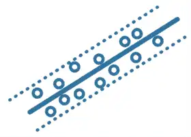 |
SVM regression algorithms work like SVM classification algorithms but are modified to be able to predict a continuous response. Instead of finding a hyperplane that separates data, SVM regression algorithms find a model that deviates from the measured data by a value no greater than a small amount, with parameter values that are as small as possible (to minimize sensitivity to error). | fitrsvm |
Understanding Support Vector Machine Regression (Documentation) Fitting an SVM Machine Learning Model (Code Example) |
| Generalized Linear Model | 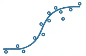 |
A generalized linear model is a special case of nonlinear models that uses linear methods. It involves fitting a linear combination of the inputs to a nonlinear function (the link function) of the outputs. | fitglm |
Generalized Linear Models (Documentation) Fitting a Generalized Linear Model (Code Example) |
| Regression Tree | 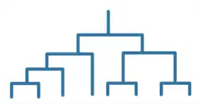 |
Decision trees for regression are similar to decision trees for classification, but they are modified to be able to predict continuous responses. | fitrtree |
Growing Decision Trees (Documentation) Fitting a Regression Tree Machine Learning Model (Code Example) |
|
Neural Network (Shallow) |
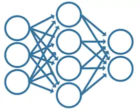 |
Inspired by the human brain, a neural network consists of highly connected networks of neurons that relate the inputs to the desired outputs. The network is trained by iteratively modifying the strengths of the connections so that training inputs map to the training responses. | fitrnet |
Neural Network Architectures (Documentation) Fitting a Neural Network Machine Learning Model (Code Example) |
| Neural Network (Deep) |  |
Deep neural networks have more hidden layers than shallow neural networks, with some instances having hundreds of hidden layers. Deep neural networks can be configured to solve regression problems by placing a regression output layer at the end of the network. | trainNetwork |
Deep Learning in MATLAB (Documentation) Fitting a Deep Neural Network for Regression (Code Example) |
| Regression Tree Ensembles | 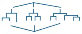 |
In ensemble methods, several “weaker” regression trees are combined into a “stronger” ensemble. The final model uses a combination of predictions from the “weaker” regression trees to calculate the final prediction. | fitrensemble |
Ensemble Algorithms (Documentation) Fitting a Regression Tree Ensemble Machine Learning Model (Code Example) |
Popular Machine Learning Models for Classification
| Model | Image | How It Works | MATLAB Function | Further Reading |
|---|---|---|---|---|
| Logistic Regression | 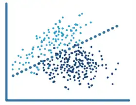 |
Logistic regression is a model that can predict the probability of a binary response belonging to one class or the other. Because of its simplicity, logistic regression is commonly used as a starting point for binary classification problems. | fitglm |
Generalized Linear Models (Documentation) Fitting a Logistic Regression Machine Learning Model (Code Example) |
| Decision Tree | 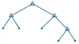 |
A decision tree lets you predict responses to data by following the decisions in the tree from the root (beginning) down to a leaf node. A tree consists of branching conditions where the value of a predictor is compared to a trained weight. The number of branches and the values of weights are determined in the training process. Additional modification, or pruning, may be used to simplify the model. | fitctree |
Growing Decision Trees (Documentation) Fitting a Decision Tree Machine Learning Model (Code Example) |
| k Nearest Neighbor (kNN) | 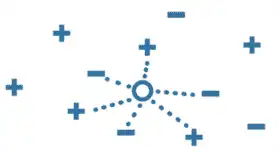 |
kNN is a type of machine learning model that categorizes objects based on the classes of their nearest neighbors in the dataset. kNN predictions assume that objects near each other are similar. Distance metrics, such as Euclidean, city block, cosine, and Chebyshev, are used to find the nearest neighbor. | fitcknn |
Classification Using Nearest Neighbors (Documentation) Fitting a k Nearest Neighbor Machine Learning Model (Code Example) |
| Support Vector Machine (SVM) | 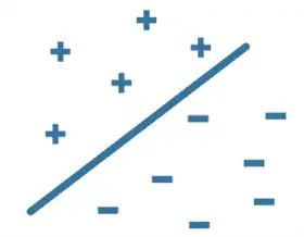 |
An SVM classifies data by finding the linear decision boundary (hyperplane) that separates all data points of one class from those of the other class. The best hyperplane for an SVM is the one with the largest margin between the two classes, when the data is linearly separable. If the data is not linearly separable, a loss function is used to penalize points on the wrong side of the hyperplane. SVMs sometimes use a kernel transform to transform nonlinearly separable data into higher dimensions where a linear decision boundary can be found. | fitcsvm |
Support Vector Machines for Binary Classification (Documentation) Fitting an SVM Machine Learning Model (Code Example) |
| Neural Network (Shallow) |  |
Inspired by the human brain, a neural network consists of highly connected networks of neurons that relate the inputs to the desired outputs. The machine learning model is trained by iteratively modifying the strengths of the connections so that given inputs map to the correct response. The neurons in between the input and output layers of a neural network are said to be in “hidden layers.” Shallow neural networks typically have one to two hidden layers. | fitcnet |
Neural Network Architectures (Documentation) Fitting a Shallow Neural Network Machine Learning Model (Code Example) |
| Neural Network (Deep) |  |
Deep neural networks have more hidden layers than shallow neural networks, with some instances having hundreds of hidden layers. Deep neural networks can be configured to solve classification problems by placing a classification output layer at the end of the network. Many pretrained deep learning models for classification are publicly available for tasks such as image recognition. | trainNetwork |
Deep Learning in MATLAB (Documentation) Fitting a Deep Neural Network Classification Model (Code Example) |
| Bagged and Boosted Decision Trees |  |
In these ensemble methods, several “weaker” decision trees are combined into a “stronger” ensemble. A bagged decision tree consists of trees that are trained independently on data that is bootstrapped from the input data. Boosting involves creating a strong learner by iteratively adding “weak” learners and adjusting the weight of each “weak” learner to focus on misclassified examples. |
fitcensemble |
Ensemble Algorithms (Documentation) Fitting a Boosted Decision Tree Ensemble (Code Example) |
| Naive Bayes |  |
A naive Bayes classifier assumes that the presence of a particular feature in a class is unrelated to the presence of any other feature. It classifies new data based on the highest probability of its belonging to a particular class. | fitcnb |
Naive Bayes Classification (Documentation) Fitting a Naive Bayes Machine Learning Model (Code Example) |
| Discriminant Analysis Ensembles | 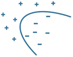 |
Discriminant analysis classifies data by finding linear combinations of features. Discriminant analysis assumes that different classes generate data based on Gaussian distributions. Training a discriminant analysis model involves finding the parameters for a Gaussian distribution for each class. The distribution parameters are used to calculate boundaries, which can be linear or quadratic functions. These boundaries are used to determine the class of new data. | fitcdiscr |
Creating Discriminant Analysis Model (Documentation) Fitting a Discriminant Analysis Machine Learning Model (Code Example) |