Filtering Data With Signal Processing Toolbox Software

Lowpass FIR Filter – Window Method

This example shows how to design and implement an FIR filter using two command line functions, fir1 and designfilt, and the interactive Filter Designer app.

Create a signal to use in the examples. The signal is a 100 Hz sine wave in additive N(0,1/4) white Gaussian noise. Set the random number generator to the default state for reproducible results.

rng default

Fs = 1000;
t = linspace(0,1,Fs);
x = cos(2*pi*100*t)+0.5*randn(size(t));

The filter design is an FIR lowpass filter with order equal to 20 and a cutoff frequency of 150 Hz. Use a Kaiser window with length one sample greater than the filter order and β=3. See kaiser for details on the Kaiser window.

Use fir1 to design the filter. fir1 requires normalized frequencies in the interval [0,1], where 1 corresponds to π rad/sample. To use fir1, you must convert all frequency specifications to normalized frequencies.

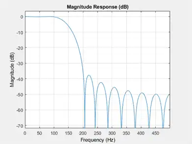
Design the filter and view the filter's magnitude response.

fc = 150;
Wn = (2/Fs)*fc;
b = fir1(20,Wn,'low',kaiser(21,3));

fvtool(b,1,'Fs',Fs)

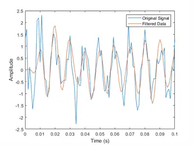
Apply the filter to the signal and plot the result for the first ten periods of the 100 Hz sinusoid.

y = filter(b,1,x);

plot(t,x,t,y)
xlim([0 0.1])

xlabel('Time (s)')
ylabel('Amplitude')
legend('Original Signal','Filtered Data')

Design the same filter using designfilt. Set the filter response to 'lowpassfir' and input the specifications as Name,Value pairs. With designfilt, you can specify your filter design in Hz.

Fs = 1000;
Hd = designfilt('lowpassfir','FilterOrder',20,'CutoffFrequency',150, ...
       'DesignMethod','window','Window',{@kaiser,3},'SampleRate',Fs);

Filter the data and plot the result.

y1 = filter(Hd,x);

plot(t,x,t,y1)
xlim([0 0.1])

xlabel('Time (s)')
ylabel('Amplitude')
legend('Original Signal','Filtered Data')

Lowpass FIR Filter with Filter Designer

This example shows how to design and implement a lowpass FIR filter using the window method with the interactive Filter Designer app.

y2 = filter(Hd,x);

plot(t,x,t,y2)
xlim([0 0.1])

xlabel('Time (s)')
ylabel('Amplitude')
legend('Original Signal','Filtered Data')

You can also use the interactive tool filterBuilder to design your filter.

Bandpass Filters – Minimum-Order FIR and IIR Systems

This example shows how to design a bandpass filter and filter data with minimum-order FIR equiripple and IIR Butterworth filters. You can model many real-world signals as a superposition of oscillating components, a low-frequency trend, and additive noise. For example, economic data often contain oscillations, which represent cycles superimposed on a slowly varying upward or downward trend. In addition, there is an additive noise component, which is a combination of measurement error and the inherent random fluctuations in the process.

In these examples, assume you sample some process every day for one year. Assume the process has oscillations on approximately one-week and one-month scales. In addition, there is a low-frequency upward trend in the data and additive N(0,1/4) white Gaussian noise.

Create the signal as a superposition of two sine waves with frequencies of 1/7 and 1/30 cycles/day. Add a low-frequency increasing trend term and N(0,1/4) white Gaussian noise. Reset the random number generator for reproducible results. The data is sampled at 1 sample/day. Plot the resulting signal and the power spectral density (PSD) estimate.

rng default

Fs = 1;
n = 1:365;

x = cos(2*pi*(1/7)*n)+cos(2*pi*(1/30)*n-pi/4);
trend = 3*sin(2*pi*(1/1480)*n);

y = x+trend+0.5*randn(size(n));

[pxx,f] = periodogram(y,[],[],Fs);

subplot(2,1,1)
plot(n,y)
xlim([1 365])
xlabel('Days')
grid

subplot(2,1,2)
plot(f,10*log10(pxx))
xlabel('Cycles/day')
ylabel('dB')
grid

The low-frequency trend appears in the power spectral density estimate as increased low-frequency power. The low-frequency power appears approximately 10 dB above the oscillation at 1/30 cycles/day. Use this information in the specifications for the filter stopbands.

Design minimum-order FIR equiripple and IIR Butterworth filters with the following specifications: passband from [1/40,1/4] cycles/day and stopbands from [0,1/60] and [1/4,1/2] cycles/day. Set both stopband attenuations to 10 dB and the passband ripple tolerance to 1 dB.

Hd1 = designfilt('bandpassfir', ...
    'StopbandFrequency1',1/60,'PassbandFrequency1',1/40, ...
    'PassbandFrequency2',1/4 ,'StopbandFrequency2',1/2 , ...
    'StopbandAttenuation1',10,'PassbandRipple',1, ...
    'StopbandAttenuation2',10,'DesignMethod','equiripple','SampleRate',Fs);
Hd2 = designfilt('bandpassiir', ...
    'StopbandFrequency1',1/60,'PassbandFrequency1',1/40, ...
    'PassbandFrequency2',1/4 ,'StopbandFrequency2',1/2 , ...
    'StopbandAttenuation1',10,'PassbandRipple',1, ...
    'StopbandAttenuation2',10,'DesignMethod','butter','SampleRate',Fs);

Compare the order of the FIR and IIR filters and the unwrapped phase responses.

fprintf('The order of the FIR filter is %d\n',filtord(Hd1))

The order of the FIR filter is 78

fprintf('The order of the IIR filter is %d\n',filtord(Hd2))

The order of the IIR filter is 8

[phifir,w] = phasez(Hd1,[],1);
[phiiir,w] = phasez(Hd2,[],1);

figure
plot(w,unwrap(phifir))
hold on
plot(w,unwrap(phiiir))
hold off

xlabel('Cycles/Day')
ylabel('Radians')
legend('FIR Equiripple Filter','IIR Butterworth Filter')
grid

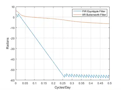
The IIR filter has a much lower order that the FIR filter. However, the FIR filter has a linear phase response over the passband, while the IIR filter does not. The FIR filter delays all frequencies in the filter passband equally, while the IIR filter does not.

Additionally, the rate of change of the phase per unit of frequency is greater in the FIR filter than in the IIR filter.

Design a lowpass FIR equiripple filter for comparison. The lowpass filter specifications are: passband [0,1/4] cycles/day, stopband attenuation equal to 10 dB, and the passband ripple tolerance set to 1 dB.

Hdlow = designfilt('lowpassfir', ...
    'PassbandFrequency',1/4,'StopbandFrequency',1/2, ...
    'PassbandRipple',1,'StopbandAttenuation',10, ...
    'DesignMethod','equiripple','SampleRate',1);

Filter the data with the bandpass and lowpass filters.

yfir = filter(Hd1,y);
yiir = filter(Hd2,y);
ylow = filter(Hdlow,y);

Plot the PSD estimate of the bandpass IIR filter output. You can replace yiir with yfir in the following code to view the PSD estimate of the FIR bandpass filter output.

[pxx,f] = periodogram(yiir,[],[],Fs);

plot(f,10*log10(pxx))

xlabel('Cycles/day')
ylabel('dB')
grid

The PSD estimate shows the bandpass filter attenuates the low-frequency trend and high-frequency noise.

Plot the first 120 days of FIR and IIR filter output.

plot(n,yfir,n,yiir)

axis([1 120 -2.8 2.8])
xlabel('Days')
legend('FIR bandpass filter output','IIR bandpass filter output', ...
    'Location','SouthEast')

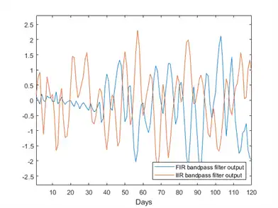
The increased phase delay in the FIR filter is evident in the filter output.

Plot the lowpass FIR filter output superimposed on the superposition of the 7-day and 30-day cycles for comparison.

plot(n,x,n,ylow)

xlim([1 365])
xlabel('Days')
legend('7-day and 30-day cycles','FIR lowpass filter output', ...
    'Location','NorthWest')

You can see in the preceding plot that the low-frequency trend is evident in the lowpass filter output. While the lowpass filter preserves the 7-day and 30-day cycles, the bandpass filters perform better in this example because the bandpass filters also remove the low-frequency trend.

Zero-Phase Filtering

This example shows how to perform zero-phase filtering.

Repeat the signal generation and lowpass filter design with fir1 and designfilt. You do not have to execute the following code if you already have these variables in your workspace.

rng default

Fs = 1000;
t = linspace(0,1,Fs);
x = cos(2*pi*100*t)+0.5*randn(size(t));

% Using fir1
fc = 150;
Wn = (2/Fs)*fc;
b = fir1(20,Wn,'low',kaiser(21,3));

% Using designfilt
Hd = designfilt('lowpassfir','FilterOrder',20,'CutoffFrequency',150, ...
       'DesignMethod','window','Window',{@kaiser,3},'SampleRate',Fs);

Filter the data using filter. Plot the first 100 points of the filter output along with a superimposed sinusoid with the same amplitude and initial phase as the input signal.

yout = filter(Hd,x);
xin = cos(2*pi*100*t);

plot(t,xin,t,yout)
xlim([0 0.1])

xlabel('Time (s)')
ylabel('Amplitude')
legend('Input Sine Wave','Filtered Data')
grid

Looking at the initial 0.01 seconds of the filtered data, you see that the output is delayed with respect to the input. The delay appears to be approximately 0.01 seconds, which is almost 1/2 the length of the FIR filter in samples (10×0.001).

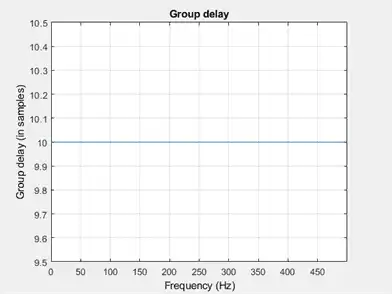
This delay is due to the filter's phase response. The FIR filter in these examples is a type I linear-phase filter. The group delay of the filter is 10 samples.

Plot the group delay using fvtool.

fvtool(Hd,'Analysis','grpdelay')

In many applications, phase distortion is acceptable. This is particularly true when phase response is linear. In other applications, it is desirable to have a filter with a zero-phase response. A zero-phase response is not technically possibly in a noncausal filter. However, you can implement zero-phase filtering using a causal filter with filtfilt.

Filter the input signal using filtfilt. Plot the responses to compare the filter outputs obtained with filter and filtfilt.

yzp = filtfilt(Hd,x);

plot(t,xin,t,yout,t,yzp)

xlim([0 0.1])
xlabel('Time (s)')
ylabel('Amplitude')
legend('100-Hz Sine Wave','Filtered Signal','Zero-phase Filtering',...
    'Location','NorthEast')

In the preceding figure, you can see that the output of filtfilt does not exhibit the delay due to the phase response of the FIR filter.